Section 4 Case 2

We illustrate how to perform integrative analysis combining genetic interactions and gene expression data; such strategy is computationally promising given the current technological limits in experimentally generating tissue-specific interactions on a genome scale, particularly for humans. One way doing so is to trim the generic genetic interactions to node genes expressed in a specific tissue. Such trimming allows identification of a genetic interaction network in the whole blood (Step 2), from which a subnetwork with a desired number of interconnected genes is further identified that tend to be highly expressed (Step 3). We also demonstrate how to highlight the subnetwork within the parent network (Step 4). For the interpretation of the subnetwork identified, we illustrate how to perform phenotype enrichment analysis using mammalian phenotype ontology, a tree-like structure containing well-defined terms that are used to annotate mouse knock-out phenotypes (Step 6).

Step 1: Load the packages and import human genetic interaction data as well as gene expression data (see Materials).

# load packages used in this case
library(tidyverse)
library(igraph)
library(XGR)
library(ggrepel)

# also load the package "osfr" aided in importing data from https://osf.io/gskpn
library(osfr)
guid <- "gskpn"

# import genetic interaction data
# converted into two tibbles "nodes" and "edges"
ig.BioGRID_genetic <- xRDataLoader("ig.BioGRID_genetic", guid=guid)
ig.BioGRID_genetic %>% igraph::as_data_frame("vertices") %>% as_tibble() -> nodes
ig.BioGRID_genetic %>% igraph::as_data_frame("edges") %>% as_tibble() -> edges

# import gene expression data
GTEx_V8_TPM_boxplot <- xRDataLoader("GTEx_V8_TPM_boxplot", guid=guid)

Step 2. Identify a genetic interaction network in the whole blood (FIGURE 4.1).

# extract genes expressed in the whole blood (TPM>=1 in all samples analysed)
# also extract median TPM among all blood samples
# stored in a tibble "df_blood"
GTEx_V8_TPM_boxplot %>% filter(SMTSD=="Whole Blood", ymin>=1) %>% 
select(Symbol,middle) -> df_blood

# trim the genetic interactions to node genes expressed
# return two data frames "vertices" and "links"
# return an igraph object "ig_blood"
edges %>% semi_join(df_blood, by=c("from"="Symbol")) %>% 
semi_join(df_blood, by=c("to"="Symbol")) %>% as.data.frame() -> links
nodes %>% inner_join(df_blood, by=c("name"="Symbol")) %>% 
rename(TPM=middle) %>% as.data.frame() -> vertices
ig_blood <- igraph::graph_from_data_frame(d=links, directed=F, vertices=vertices)

# calculate coordinates using the Fruchterman-Reingold layout algorithm
# the object "ig_blood" appended with two node attributes "xcoord" and "ycoord" 
ig_blood %>% xLayout("gplot.layout.fruchtermanreingold") -> ig_blood

# calculate node degree (the number of neighbors) 
# the object "ig_blood" appended with a node attribute "degree" 
igraph::degree(ig_blood) -> V(ig_blood)$degree

# visualise the network
# nodes placed by coordinates
# nodes sized by degree
# sizebar hidden
# return a ggplot object "gg_blood"
ig_blood %>% xGGnetwork(node.xcoord="xcoord", node.ycoord="ycoord", node.size="degree", node.size.range=c(0.5,2.5), edge.color="lightblue1", edge.arrow.gap=0) + 
guides(size="none") -> gg_blood
gg_blood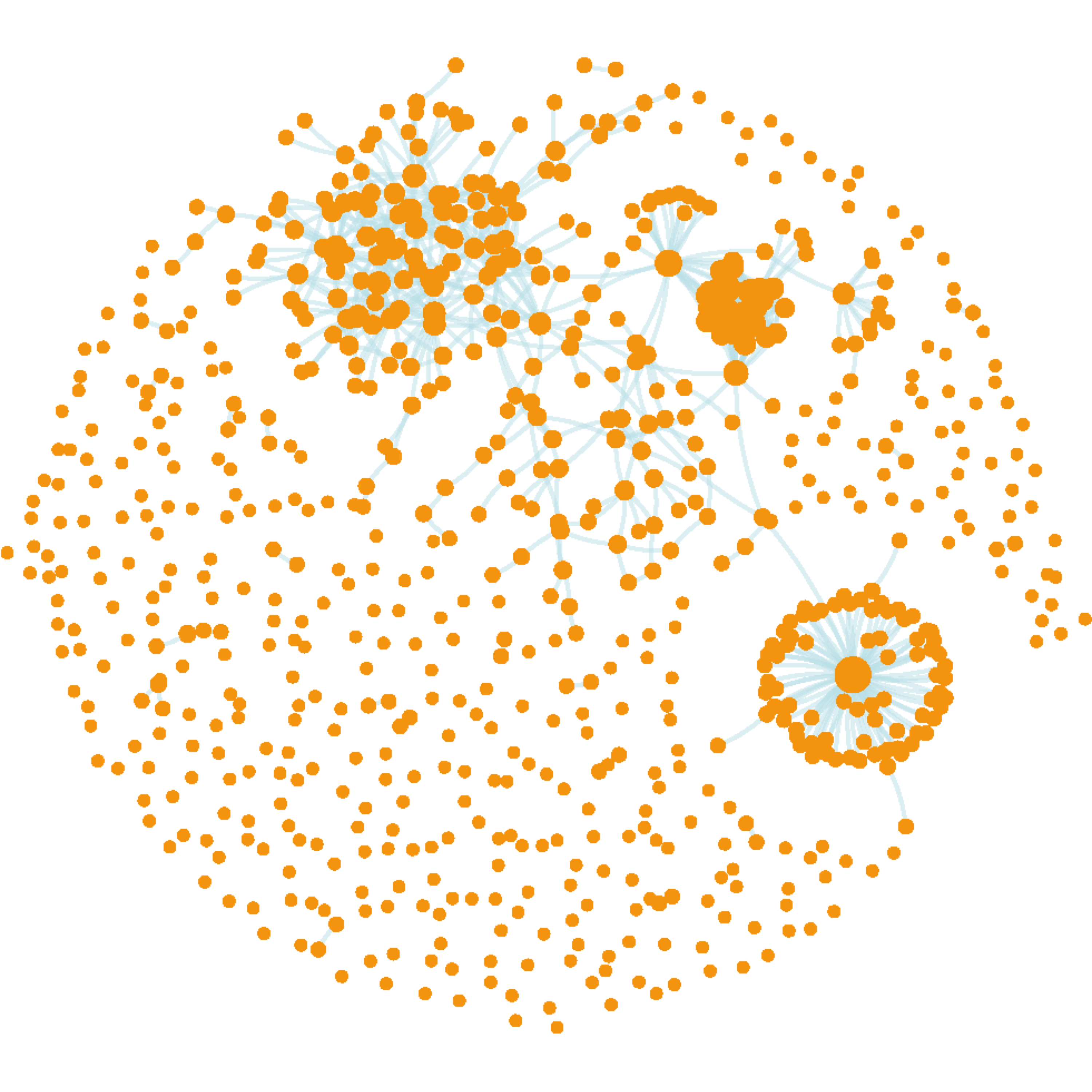

FIGURE 4.1: Network visualisation of genetic interactions containing 756 nodes/genes (expressed in the human whole blood) and 725 edges (notably, not all interconnected). Nodes sized by degree (i.e. the number of interacting neighbors).

Step 3: Further identify a subnetwork with highly expressed genes (FIGURE 4.2).

# weight nodes by expression (TPM), the higher the more weight
# transform the weight into a p-value-like quantity
# thus, a node with the higher expression receives a lower p-value
vertices %>% 
mutate(x=log10(TPM), x=100*(x-min(x))/(max(x)-min(x)), pval=10^(-x)) %>% 
select(symbol,pval) %>% as.data.frame -> data

# identify a subnetowrk with a desired number (~30) of interconnected genes
# return an igraph object "ig_subg"
data %>% xSubneterGenes(network.customised=ig_blood, subnet.size=30) -> ig_subg

# the object "ig_subg" appended with a node attribute "TPM"
ind <- match(V(ig_subg)$name, vertices$symbol)
V(ig_subg)$TPM <- log10(vertices$TPM[ind])

# the object "ig_subg" appended with two node attributes "xcoord" and "ycoord"
# based on node coordinates in the object 'ig_blood'
ind <- match(V(ig_subg)$name, V(ig_blood)$name)
V(ig_subg)$xcoord <- V(ig_blood)$xcoord[ind]
V(ig_subg)$ycoord <- V(ig_blood)$ycoord[ind]

# visualise the subnetwork
# nodes labelled by gene names
# nodes placed by coordinates
# nodes colored by TPM
# return a ggplot object "gg_subg"
ig_subg %>% xGGnetwork(node.label="name", node.label.size=2, node.label.color="black", node.label.force=0.05, node.xcoord="xcoord", node.ycoord="ycoord", node.color="TPM", node.color.title=expression(log[10]("median TPM")), colormap="brewer.Greens", zlim=c(0,4), edge.color="lightblue", edge.arrow.gap=0) -> gg_subg
gg_subg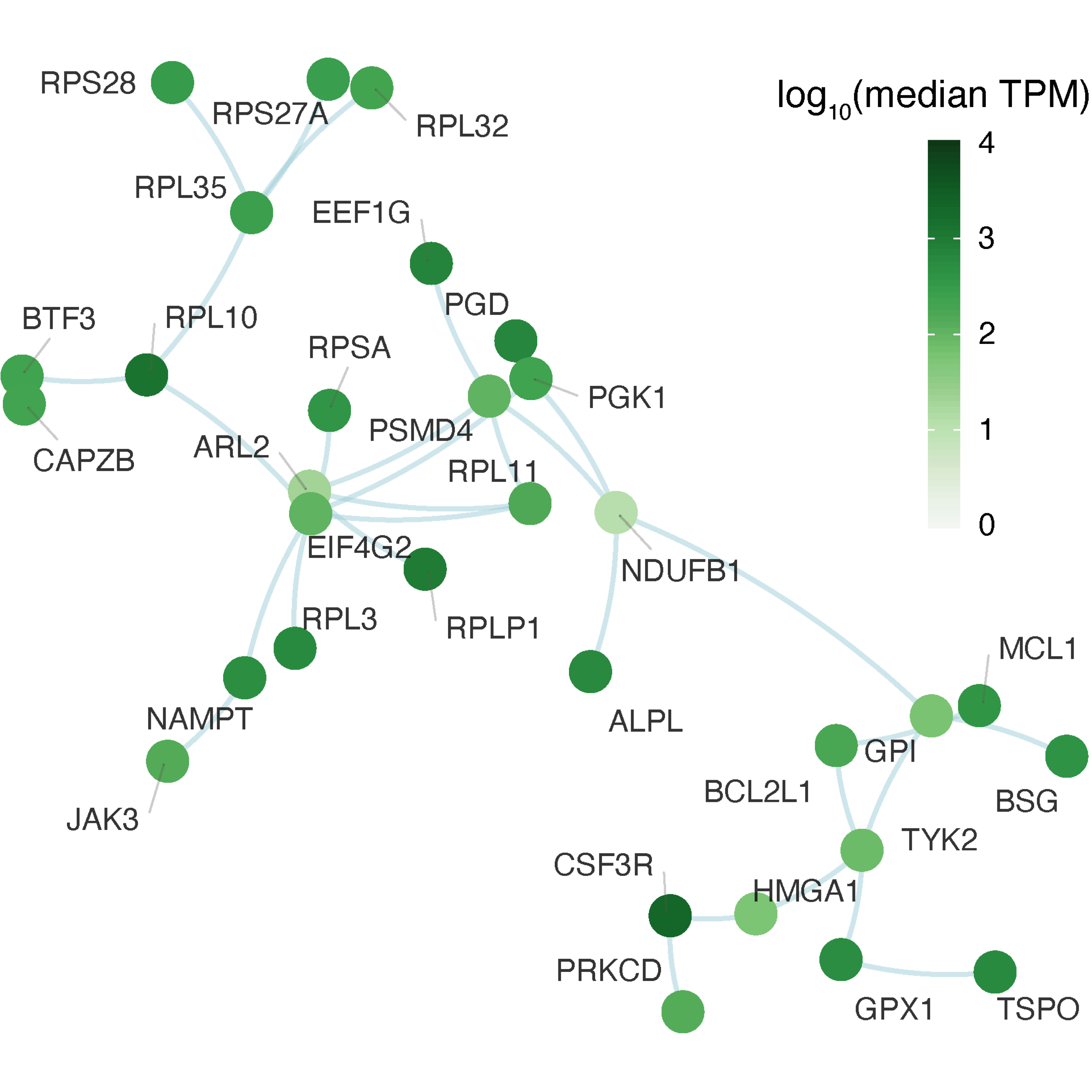

FIGURE 4.2: Illustration of a subnetwork identified from the parent network, ensuring the subnetwork has a desired number (here ~30) of interconnected nodes/genes that tend to be highly expressed in the whole blood. Nodes colored by the median expression level, that is, transcripts per million (TPM).

Step 4. Highlight the subnetwork within the parent network.

# the "ig_blood" (the parent network) marked by the "ig_subg" (the subnetwork)
# return an igraph object "ig_blood2", the same as "ig_blood"
# but appended with a node attribute ("mark") and an edge attribute ("mark") 
ig_blood2 <- xMarkNet(ig_blood, ig_subg)

# the object "ig_blood2" appended with two node attributes "xcoord" and "ycoord" 
# coordinates calculated using the Fruchterman-Reingold layout algorithm
ig_blood2 %>% xLayout("gplot.layout.fruchtermanreingold") -> ig_blood2

# the object "ig_blood2" appended with two edge attributes
# "color" for edge coloring and "color.alpha" for edge color transparency
E(ig_blood2)$color <- ifelse(E(ig_blood2)$mark==0, "lightblue1", "darkgreen")
E(ig_blood2)$color.alpha <- ifelse(E(ig_blood2)$mark==0, 0.3, 0.9)

# visualise the parent network highlighted by the subnetwork
# nodes placed by coordinates
# nodes sized by degree
# nodes colored differently, thus, being highlighted
# edges colored differently, thus, being highlighted
# return a ggplot object "gg_blood2"
ig_blood2 %>% xGGnetwork(node.xcoord="xcoord", node.ycoord="ycoord", , node.size="degree", node.size.range=c(0.5,2.5), node.color="mark", colormap="orange-darkgreen", node.color.alpha=0.7, edge.color="color", edge.color.alpha="color.alpha", edge.arrow.gap=0) + guides(size="none") + guides(color="none") -> gg_blood2
gg_blood2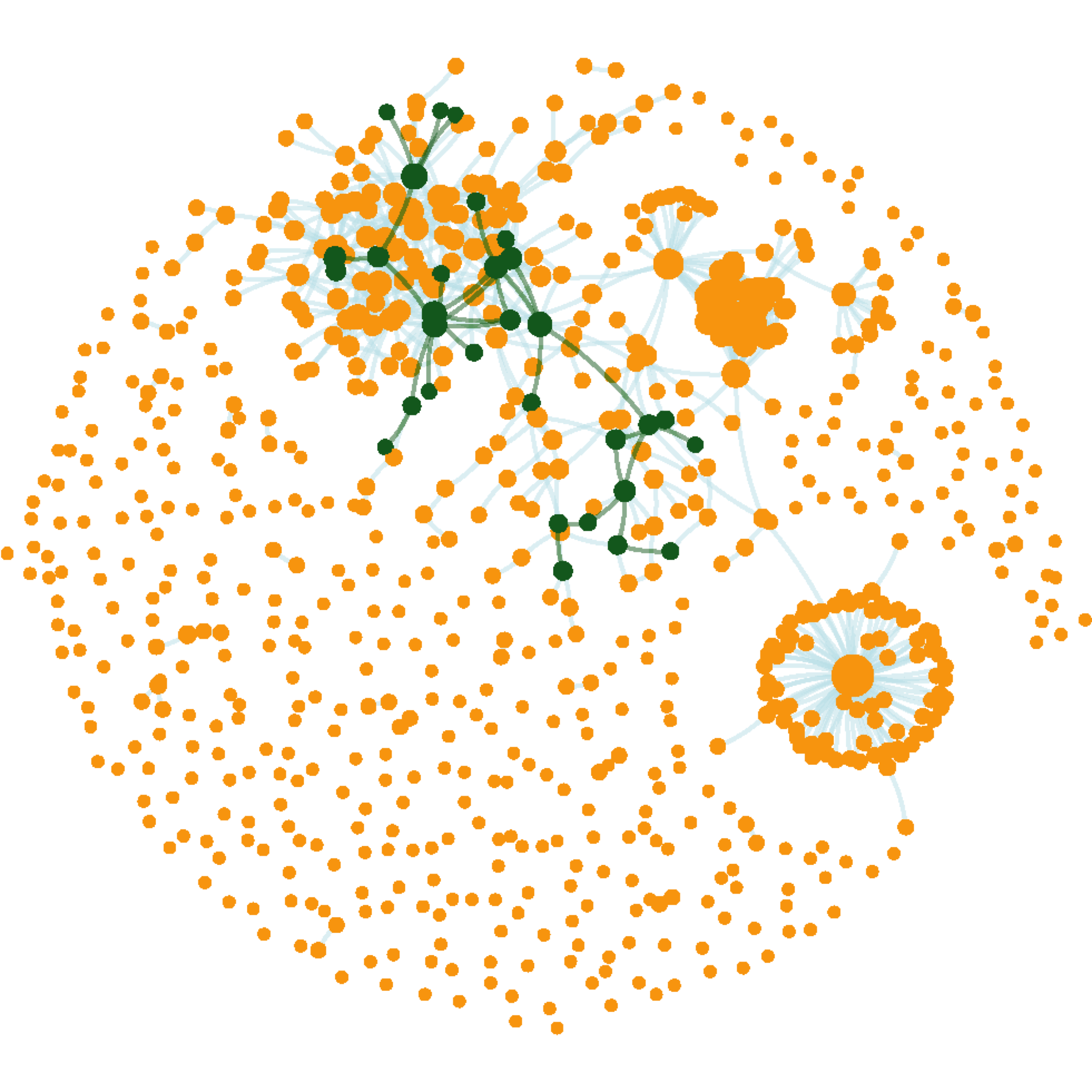

FIGURE 4.3: The parent network highlighted with the subnetwork. The layout (node coordinates) preserved.

Step 5. Display expression levels for genes in the subnetwork (FIGURE 4.4).

# extract whole blood expression data for genes in the subnetwork
GTEx_V8_TPM_boxplot %>% 
filter(SMTSD %in% c("Whole Blood"), Symbol %in% V(ig_subg)$name) -> data

# genes ordered by median expression level, converted into a factor
data %>% arrange(middle) %>% mutate(Symbol=fct_inorder(Symbol)) -> data

# draw the boxplot, showing the distribution among the blood samples
data %>% ggplot(aes(x=Symbol)) + geom_boxplot(stat="identity", aes(ymin=ymin,lower=lower,middle=middle,upper=upper,ymax=ymax), fill="green3") + ylab("TPM") + xlab("") + scale_y_log10() + coord_flip() + theme_minimal()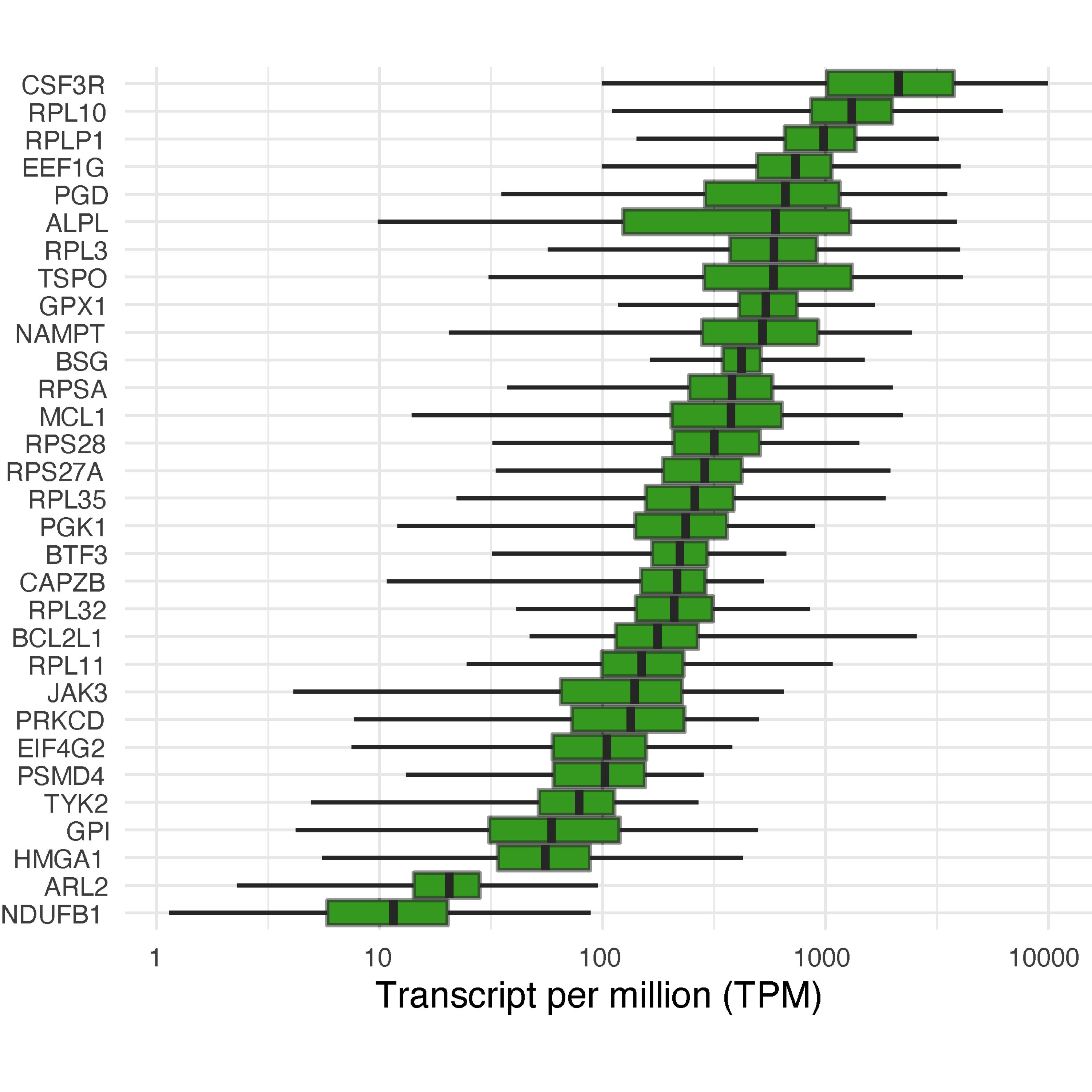

FIGURE 4.4: Boxplot of genes in the subnetwork, showing expression distribution across the whole blood samples.

Step 6. Perform phenotype enrichment analysis for genes in the subnetwork (FIGURE 4.5).

# define the test background (all genes expressed in the whole blood)
GTEx_V8_TPM_boxplot %>% filter(SMTSD=="Whole Blood", ymin>=1) %>% 
pull(Symbol) -> background

# perform enrichment analysis using mammalian phenotype ontology
# return an eTerm object "eTerm"
V(ig_subg)$name %>% xEnricherGenes(background=background, ontology="MP", guid=guid) -> eTerm

# circular visualisation of enriched phenotypes within the ontology 
eTerm %>% xEnrichGGraph(fixed=F, node.label.direction="leftright", slim=c(1,3))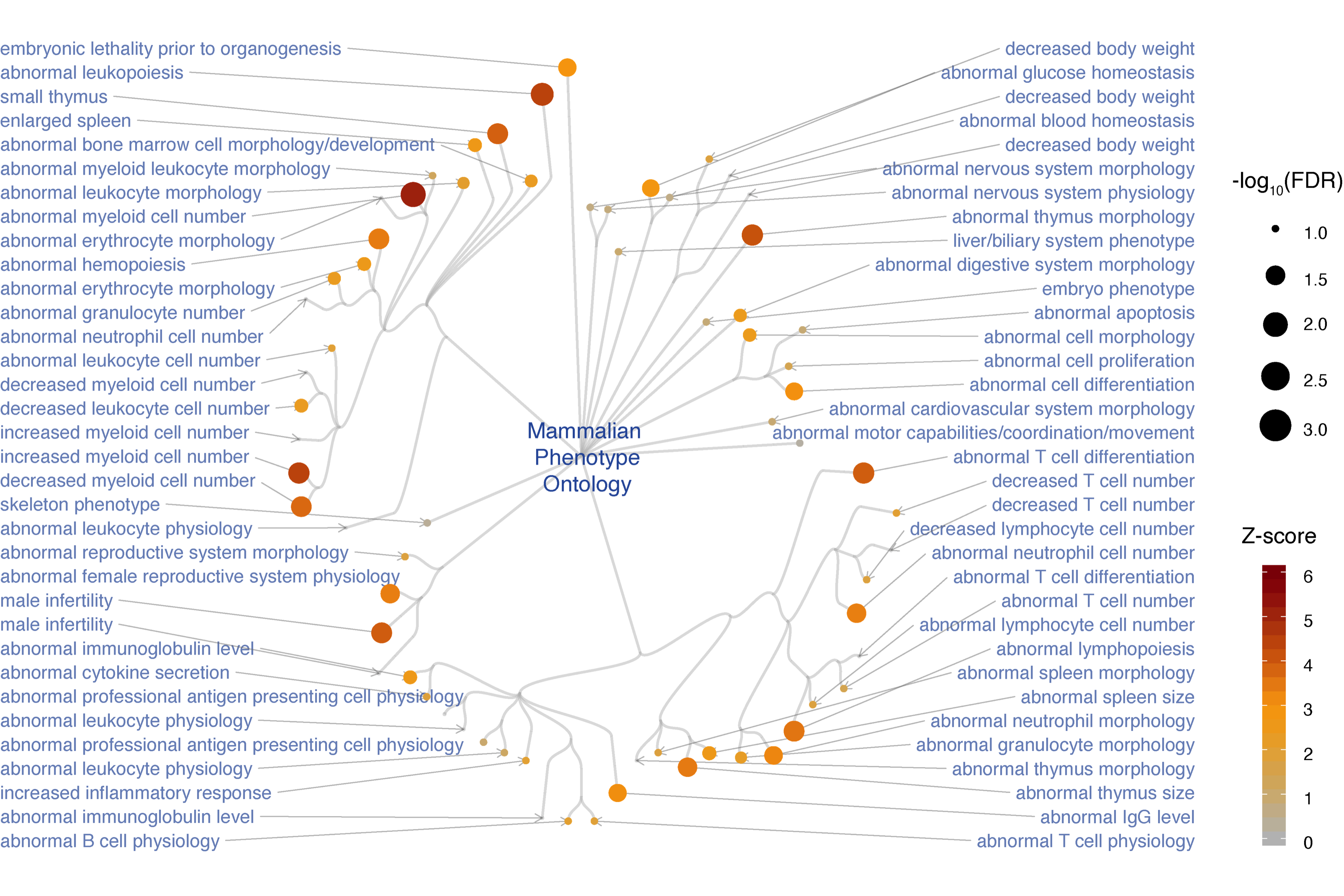

FIGURE 4.5: Circular illustration of mouse phenotypes enriched in subnetwork genes. Based on mammalian phenotype ontology used for annotating mouse knockout genes.